Multi-Dimensional Optimization: A Better Goal Seek

The code for the examples can be found in the optimization folder of our examples repository.

Improving on Excel’s Solver with Python

Excel comes with an installable add-in called the solver, which is admirably well-suited to general optimization problems. You will find a simple description of the solver’s capabilities in this series of articles. This is a perfectly satisfactory way to solve many relatively simple models. In spreadsheet work the objective function is typically some model describing real-world objects and relationships between them.

Although versatile, like most packaged software the solver has its limitations (limited choice of strategies, problem size and constraint size limitations being the most frequent issues), and so at some stage you may well find that you would like Excel to optimize models that are currently outside its capabilities.

PyXLL users can deploy Python-based solutions to extend Excel’s optimization abilities in any number of ways, tailored as necessary to their specific problems.

In this article we consider how to make use of the many advanced optimization facilities readily available in the open source scipy.optimize library. As a glance at that listing clearly shows there are optimization routines available to cope with all kinds of circumstances.

Optimization principles

Optimization is very simple in principle. Then again, so is juggling, but the practice turns out to be rather difficult and far less straightforward than it seems in theory.

Any process of optimization requires the finding of a minimum or maximum value for some function (the so-called objective function) that produces a scalar output (to avoid ambiguity in maximisation). The difficulty of the problem is primarily determined by the dimensionality of the problem: the number of scalar values in the function’s input.

Starting with chosen initial values the optimizer varies the inputs to the objective function to either maximise or minimise its value. A feedback loop directs the changes in the inputs according to the strategy the optimizer uses and the results of earlier evaluations.  This relatively simple statement, however, can hide a multitude of complexities.

They arrive in the form of questions such as these:

• What is an efficient strategy for this particular optimization?
• What guarantees are there that the selected optimum is indeed optimal?
• What constraints can the optimizer accept on the inputs?

Using Python to optimize in Excel

While the solver can offer a good first handle on an optimization problem, it cannot hope to offer the sophistication of the many different techniques available in the scipy.optimize library, which offers specialised methods for particular types of problem, and efficiency improvements when more is known about the function (for example, if we know the function’s slope at a current evaluation point this allows us to make better guesses about more optimal values for the inputs).

Scipy’s optimization tutorial demonstrates several uses of the library in Python, and will repay further study. As those examples make clear, the best solution to a complex optimization problem often requires some study and experimentation. This post gives you the information you will need to do the necessary experimentation.

Creating the Excel objective function

Before you can make your spreadsheet provide the objective function for your optimization, you need to understand a little about how Excel’s calculation cycle works. Excel records each cell’s precedents (the cells on whose value this cell’s value depends) and dependents (the cells whose value depends on this cell’s value). Whenever any cell’s value is changed the value of all its dependent cells must then be recalculated, and then the values of their dependent cells, and so on until no calculation work remains.

The objective function in Excel will simply be a formula in a cell that takes one or more inputs, for which we want to find a set of inputs that produce the minimum result.

Let’s start with a very simple Excel model based on a periodic function with two inputs and a single output. Mathematically we can write that as

z = f(x, y) = sin(x)cos(y)

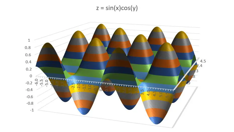
Here’s a 3-D plot of the function’s behaviour for values of x and y around the origin:

As you can see, the periodic nature of the function means that the maxima and minima repeat, so the answer you get will depend on where you start looking (the initial values for x and y).

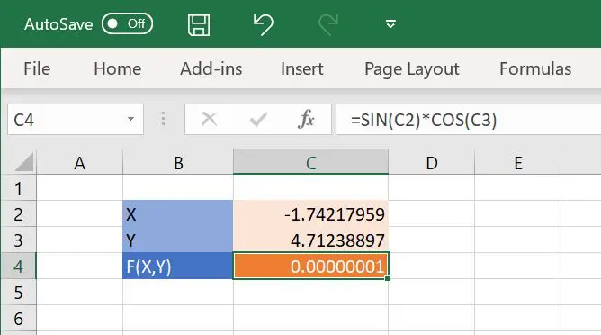
In Excel we can calculate F(X,Y) by putting our inputs X and Y in cells C2 and C3 and then the formula (our objective function) =SIN(C2)*COS(C3) in cell C4.

The techniques in scipy.optimize all rely on the optimizer being able to call an objective function written in Python, so when using an Excel model we need to wrap it to make it possible for the optimizer to call. In pseudo-code terms we might define such a function as follows (remember that in numpy, variables can be multi-dimensional, so x might be a vector that is stored in multiple cells):

def objective_function(x):
    # Set model's input(s) to x
    # Have Excel calculate the model
    # Return the value of the output cell

A simple implementation of an objective function that gets the inputs from cells C2 and C3, calculates the sheet, and reads the result from C4 is as follows:

from pyxll import xl_app

def objective_func(arg):
    xl = xl_app()
    # Copy argument values to input range
    xl.Range('C2').Value = float(arg[0])
    xl.Range('C3').Value = float(arg[1])

    # Calculate after changing the inputs
    xl.Calculate()

    # Return the value of the output cell
    result = xl.Range("C4").Value
    
    return result

Each time the function is called (with a two-element numpy array as its argument) the elements of the array are copied into the input cells, Excel is told to run a calculation cycle and the value of the result cell is returned as the value of the function call.

Solving for X and Y

Now that we have an objective function objective_func we can use scipy.optimize.minimize to solve for its minimal value. Using the Nelder-Mead algorithm a suitable line of Python would read:

from scipy.optimize import minimize

minimize(objective_func, INITIAL_VALUES, method='nelder-mead')

Here INITIAL_VALUES is the initial value for the function’s arguments. For multivariate optimization problems this should be a simple vector of type numpy.array.

To call this from Excel we can use PyXLL’s @xl_macro decorator to create an Excel macro that will call the scipy optimizer. This macro can be assigned to a button in Excel, or called via a shortcut key. We could equally well use @xl_menu or use a ribbon function if that suited our requirements better.

The macro collects the initial values from cells C2 and C3 in the sheet and calls scipy.optimize.minimize with our objective function. It also sets Excel to “Manual Calc” mode and disables screen updating while the optimization is running. Disabling screen updating is advisable for any task that does lots of updating, as refreshing the screen on each update slows things down. “Manual Calc” mode ensures that we can make multiple updates to Excel and only trigger a recalculation once all the inputs have been set. A try/finally block is used to ensure that Excel’s settings are restored before the function returns.

from pyxll import xl_macro, xl_app
from win32com.client import constants

@xl_macro(shortcut='Ctrl+Alt+P')
def optimize():
    xl = xl_app()     # Get the initial values of the input cells
    x = xl.Range("C2").Value
    y = xl.Range("C3").Value
    X = np.array([x, y])
    orig_calc_mode = xl.Calculation
    try:
        # switch Excel to manual calculation
        # and disable screen updating
        xl.Calculation = constants.xlManual
        xl.ScreenUpdating = False
        # run the minimization routine
        minimize(obj_func, X, method='nelder-mead')
    finally:
        # restore the original calculation
        # and screen updating mode
        xl.ScreenUpdating = True 
        xl.Calculation = orig_calc_mode

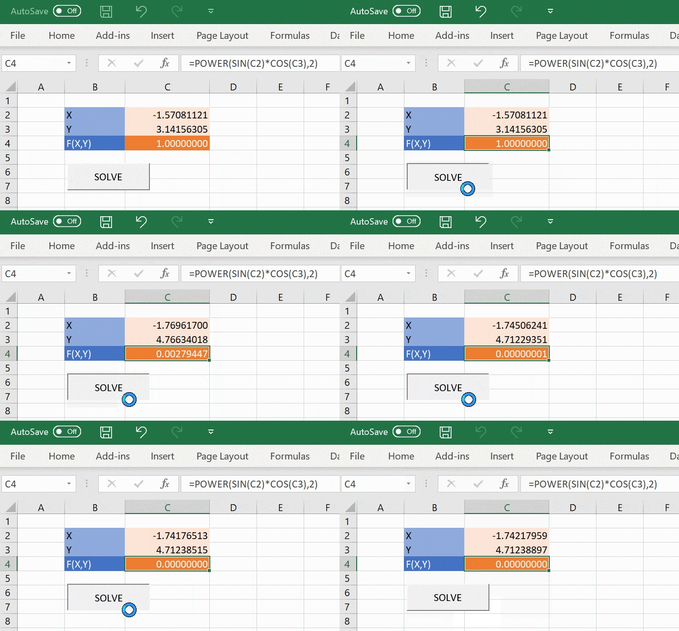
Calling this macro via the shortcut key or by assigning the macro to a button solves X and Y in cells C2 and C3 to give the minimum value of F(X,Y) in cell C4.

Further Improvements

The code as presented so far can be found in file optimize1.py in the Github repo. For larger multivariate problems it’s inconvenient to write a separate statement for each value in the function input. In the optimize2.py file this inputs are gathered by statements that will cope with a range of any size.

# Get the initial values of the input cells
in_values = xl.Range('C11:C12').Value
X = np.array([x[0] for x in in_values])

The optimize3.py file takes things a little further, using a named input range and also avoiding the need for the objective function to look up the Excel app each time it is called by making the app a parameter to the objective function and then binding it permanently using functools.partial. The objective function declaration is modified thus:

def obj_func(xl, arg):
    """Wraps a spreadsheet computation as a Python function."""
    # Copy argument values to input range
    xl.Range('Inputs').Value = [(float(x), ) for x in arg]

    # Calculate after changing the inputs
    xl.Calculate()

    # Return the value of the output cell
    result = xl.Range("Output").Value
    return result

The optimizer is modified to bind the xl argument, leaving it as the required single-argument function :

xl_obj_func = partial(obj_func, xl)
minimize(xl_obj_func, X, method='nelder-mead')

Conclusions

While the objective function demonstrated in this article is trivial, the same principles apply to any workbook where an input vector is transformed into a scalar objective measure. This allows you to broaden the scope of your optimization efforts while retaining the well-known Excel interface and all its corporate benefits.

For a more flexible solver, it would be an advantage to be able to select the inputs and output via a user interface. This can be achieved using one of Python’s UI toolkits such as PyQt5 but that is beyond the scope of this article.