Whether you’re trading for yourself or part of a large trading team, you will more than likely work with huge data sets. Whether you’re developing and refining your own technical indicators or running fully automated algorithmic trading using machine learning, having fast and easy access to accurate data sets is key. Accurate data sets are essential to your success.
Excel is still, by far, the most used and most flexible tool for working with data. But, you may well be thinking, how can you use Excel effectively when dealing with huge data sets such as intraday FX tick data? Excel is limited to just over 1 million rows, and even so, on a modern fast PC with plenty of memory it still starts to slow down way before you reach that limit.
You can manage large amounts of data in Excel, you just have to be smart about it! Collecting, cleaning and organizing the data is just part of the story. You also need the tools to work with that data. Excel can be a perfect, interactive, front-end for those tools – in just the same way you might build a web application (but with much less effort)!
Python in Excel

If you’ve been working with large data sets then you will already be using Python! Python is the most widely used programming language for data science, machine learning, and industries that use those such as Finance and Engineering.
The PyXLL Excel add-in bridges your Python code and Excel, enabling you to build custom tools to use directly in Excel or deploy to Excel users in your team (even if they have no knowledge of Python).
With PyXLL, Excel becomes a user interface toolkit for you to build out solutions in Excel. The Python code runs locally and can import all of your Python packages. You can write Python functions to be called from the workbook, in exactly the same way as Excel’s built-in functions. Because the Python code still lives outside of Excel, you can reuse the same Python code across Excel, batch processing, web apps, and everywhere else you use that code.
To get started using PyXLL, please visit https://www.pyxll.com.
If you’re new to PyXLL, this video is a great place to start https://www.pyxll.com/docs/videos/worksheet-functions.html.
Introducing ArcticDB

ArcticDB is a scalable, high performance DataFrame database developed by Man Group. It powers research and trading activity not just within Man Group but across a growing number of organizations including some of the world’s largest financial firms like Bloomberg to name just one.
One of the key features of ArcticDB is how easy it is to get up and running. Traditionally, setting up a large database requires a lot of effort and coordination with database teams, but with ArcticDB you choose where you want to store you data (even keeping it locally on your PC) and start saving pandas DataFrames to it.
To use ArcticDB in your Python environment, pip install it using the following command
pip install arcticdbPlease visit https://arcticdb.io for more details about ArcticDB and help getting started. ArcticDB is developed by Man Group, https://www.man.com.
23 Millions rows in Excel, using PyXLL and ArcticDB
To look at how we can leverage large data sets in Excel, we first need a large data set! For this example, we’re going to use a free foreign exchange intra-day tick data set from https://www.histdata.com.
Preparing the data
Begin by downloading the CSV files from https://www.histdata.com/download-free-forex-historical-data/?/ascii/tick-data-quotes/eurusd/2023. Even one month of this data is too big to be loaded into Excel!
Next, unzip each of the downloaded zip files so you have a folder of CSV files. Now we need some Python code to load each of these CSV files so we can save them to ArcticDB.
To load the CSV files I’ve used another package, polars (https://pola.rs). This is the fastest way I’ve found of reading large CSV files. If you don’t already have polars installed, you can install it by running “pip install polars”. My CSV files were located in a folder named “E:/fx-data” so you will need to change the code below to where you’ve saved the files.
import polars as pl

# Load the csv data using polars
df = pl.scan_csv("E:/fx-data/DAT_ASCII_EURUSD_T_*.csv", has_header=False)

# Extract time, bid, ask and mid (mid is calculated from bid and ask)
df = df.select(
    pl.col("column_1").alias("timestamp").str.to_datetime("%Y%m%d %H%M%S%3f", time_unit="ns"),
    pl.col("column_2").alias("bid"),
    pl.col("column_3").alias("ask"),
    (pl.col("column_2") + ((pl.col("column_3") - pl.col("column_2")) / 2)).alias("mid"),
 ).sort("timestamp", descending=False)

# Convert to pandas and ensure index is sorted
dfp = df.collect().to_pandas()
dfp = dfp.set_index("timestamp")
dfp = dfp.sort_index()
Loading the data into ArcticDB
The code above loads all of the fx data into a pandas DataFrame, “dfp”. Next we can create an ArcticDB library and save that data. Once the data is saved in ArcticDB it can be queried and retrieved quickly.
import arcticdb as adb

# Create the ArcticDB library on our local file system
ac = adb.Arctic("lmdb://E:/fx-data/arcticdb")
lib = ac.get_library("fx-test", create_if_missing=True)

# Write the DataFrame created above to the ArcticDB library
lib.write("EURUSD", dfp)
That one line at the end, lib.write("EURUSD", dfp), is all that’s needed to save our DataFrame to ArcticDB! Next we will look at how to read it back out.
Querying the data from ArcticDB
Let’s start with something simple; reading a small section of the data for a specific interval.
We first need to get the ArcticDB library object, which I’m going to write as a function since we will use that quite often:
def adb_library(url, library_name):
    ac = adb.Arctic(url)
    return ac[library_name]
Once we have the library we can access the data using the “read” method. We’ll do that in a second function which we’ll call “raw_tick_data”.
def raw_tick_data(lib, symbol, start, end):
    data = lib.read(symbol, date_range=[start, end])
    return data.data
You’ll see why I have written the above as two functions very shortly… but for now, we can call the first to get the library, and the second to get the data for a specific interval as follows:
import datetime as dt

lib = adb_library("lmdb://E:/fx-data/arcticdb", "fx-data")

start = dt.datetime(2023, 8, 3, 7, 0, 0)
end = dt.datetime(2023, 8, 3, 7, 1, 0)

data = raw_tick_data(lib, "EURUSD", start, end)
And with that simple few lines of code we’ve not got a DataFrame containing the raw tick data for a specific time interval!
Bringing ArcticDB into Excel with PyXLL
We’ve seen above how simple and fast it is to query the raw tick data for a time interval using just a little bit of Python code. Let’s face it though, it would be much more convenient if you could pull the same data up in Excel! Especially if you work as part of a wider team where many people live and breath in Excel, having tools like this at their disposal is invaluable.
To expose those two functions to Excel all we need is to install the PyXLL Excel add-in, configure the add-in to load the module we wrote above, and add the “@xl_func” decorator to the functions. The @xl_func decorator tells the PyXLL add-in we would like to call those functions in Excel.
import arcticdb as adb
from pyxll import xl_func

@xl_func("str, str: object")
def adb_library(url, library_name):
    ac = adb.Arctic(url)
    return ac[library_name]

@xl_func("object, str, datetime, datetime, int: dataframe<index=True>")
def raw_tick_data(lib, symbol, start, end):
    data = lib.read(symbol, date_range=[start, end])
    return data.data
The parameter to right of each @xl_func tells the PyXLL add-in how to convert the Excel input arguments to Python, and how to convert the Python return value to an Excel type. Other than that, you can see the code is exactly the same as before.
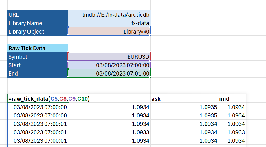
With the Python module saved, PyXLL configured to load it, and Excel started, we can call “=adb_library” from an Excel workbook and the ArcticDB Library object is returned to the sheet.

We can then pass that Library object to our “raw_tick_data” function, along with the other options for the ticker, start and end date, and load the data we need directly in Excel – no Python experience required!

We now have an amazingly quick and simple way to access huge data sets directly in Excel, pulling in only the data needed so the sheet stays small and responsive.
Making sense of tick data using resampling
Querying the raw tick data is great if we’re drilling in to a very specific time period. Other times, we want to see how the market is behaving at a higher level. By ‘resampling’ the tick data we can calculate the open, high, low and close price for regular intervals. This collapses the fine grained tick data into something much more comprehensible.
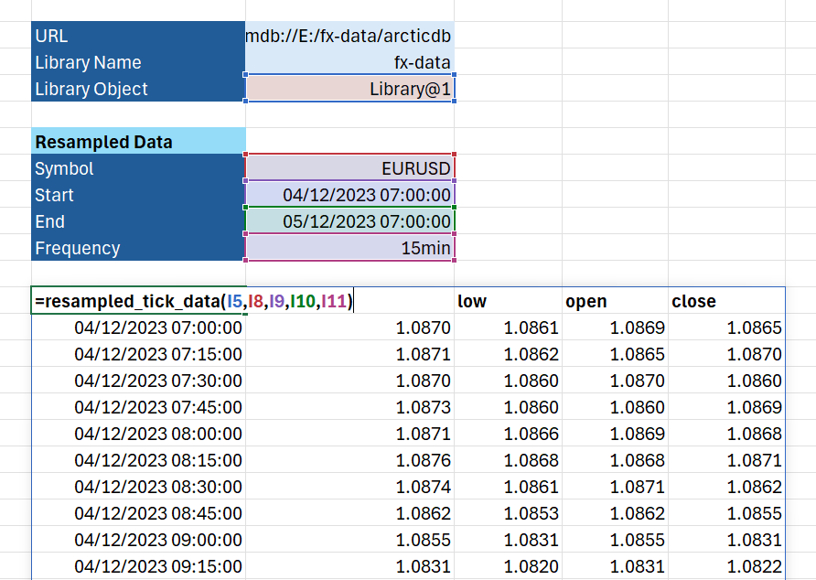
To resample our tick data into 15 minute intervals, for each 15 minute interval we record the price at the start of the interval (open); the maximum price in that interval (high); lowest price in the interval (low) and the last price in the interval (close).
ArcticDB makes resampling data in this way simple, and fast! Letting ArcticDB take care of the resampling is much more efficient than loading all of the data and doing it in Python. Once we expose that functionality to Excel the result is a super-fast tool for building interactive spreadsheets.
We’ll write a function as before to query the ArcticDB library. This time we use the QueryBuilder API to build a query that fetches the data and does the resampling in one go:
@xl_func("object, str, datetime, datetime, str, int: dataframe<index=True>")
def resampled_tick_data(lib, symbol, start, end, freq):
    qb = adb.QueryBuilder()

    qb = qb.resample(freq, closed='right').agg({
        'high': ('mid', 'max'),
        'low': ('mid', 'min'),
        'open': ('mid', 'first'),
        'close': ('mid', 'last')
    })

    data = lib.read(symbol,
                    date_range=[start, end],
                    query_builder=qb)

    df = data.data.dropna()
    return df
I’ve included the @xl_func decorator on this function as with the functions above. This is what makes this function callable from Excel. With this function added to the Python module, either reload the PyXLL add-in or restart Excel and the function will be available.
There’s a more detailed example of using resampling in the ArcticDB examples here https://docs.arcticdb.io/dev/notebooks/ArcticDB_demo_resample.

Querying and resampling data using this function in Excel is incredibly fast!
Plotting a candlestick chart in Excel
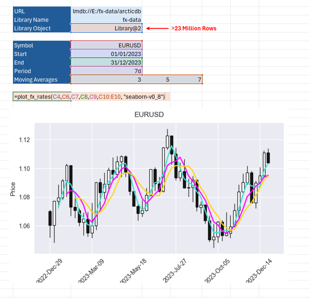
Now we’ve learned how to query and resample data we can look at ways to visualize that data. A common chart type used in finance is the “candlestick” chart. It’s exactly what we need to show the open/high/low/close (OHLC) resampled data we’ve computed above.
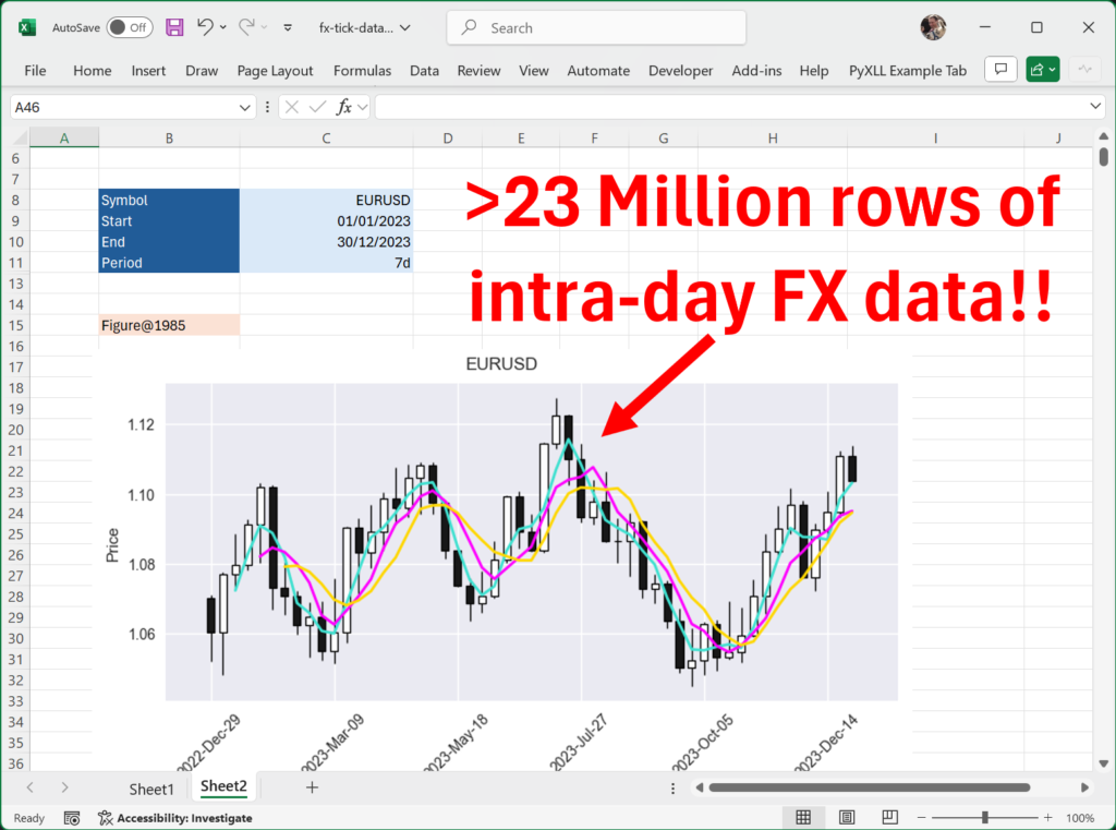
Our final function queries and resamples the data as before. But, rather than return the data to be displayed in the Excel grid, we will plot the data as a chart and display that chart in Excel.
To do this we will use two more packages, “mplfinance” and “matplotlib”. Matplotlib is a well known Python plotting library and can be used to create virtually any type of plot. To make things simple, mplfinance provides some convenience functions specific to finance, such as plotting candlestick charts.
import matplotlib.pyplot as plt
import mplfinance as mpf
import pyxll

@xl_func("object, str, datetime, datetime, str, int[], str: var")
def plot_fx_rates(lib, symbol, start, end, freq="1D", mav=[], style="seaborn-v0_8"):
    # Build the query that will get the resampled data
    qb = adb.QueryBuilder()
    qb = qb.resample(freq, closed='right').agg({
        'high': ('mid', 'max'),
        'low': ('mid', 'min'),
        'open': ('mid', 'first'),
        'close': ('mid', 'last')
    })

    # Read the data from our ArcticDB library
    df = lib.read(symbol,
        date_range=[start, end],
        query_builder=qb).data

    # Plot the candlestick chart using pyplot and mplfinance
    with plt.style.context(style):
        # Get a matplotlib Figure and Axes object to plot the candlestick chart on
        fig, ax = plt.subplots()
        fig.suptitle(symbol)
        ax.grid(True)

        # Use matplotlibfinance to draw the candlestick chart
        mpf.plot(df,
                 type='candle',
                 mav=[x for x in mav if x],
                 ax=ax)

        fig.tight_layout()

        # Show the chart in Excel
        pyxll.plot(fig)

    return fig
The PyXLL function “plot” takes the matplotlib figure and displays it in Excel, just below where the function is called. The PyXLL plot function also works with other Python plotting libraries so you can create any visualizations you need beyond the basic Excel charts, using Python.
You might have noticed the addition of the “mav” argument to the function above. This is a list of “moving averages”. The mplfinance library can draw the moving averages for us. This extra argument allows the Excel user to pass in a list of periods so they can control which moving averages get drawn.

To read more about the plotting capabilities of PyXLL, see this page in the PyXLL docs https://www.pyxll.com/docs/userguide/plotting/index.html.
Wrapping Up
In this post we’ve seen how to save and query huge data sets into the ArcticDB database. ArcticDB greatly simplifies organizing your financial tick data, or indeed any time series data you might be dealing with!
Using PyXLL, we can write tools to be used in Excel, written in Python. This allows us to take advantage of packages like ArcticDB from within Excel. By using Excel as a front-end to our Python code we massively reduce the time needed to develop interactive tools. Rather than a web app with the obligatory “Export to Excel” button, or overnight reports generating CSV files, we can have the tools we need right in Excel.
Resources
All of the code and an example workbook used in this blog post can be downloaded from here https://www.pyxll.com/blog/wp-content/uploads/2024/08/arcticdb-fx-demo.zip
- For more information about ArcticDB please visit https://arcticdb.io
- If you would like to learn more about PyXLL, please go to https://www.pyxll.com
- ArcticDB is developed by Man Group. You can find there website here https://www.man.com
For any questions please contact PyXLL support via https://www.pyxll.com/contact.html and we will be happy to assist.
